Life of Linear System
When a linear system reciprocates under loading, a continuous stress acts on it, ultimately causing flaking of its raceway surface due to material fatigue. The distance a linear system travels before this flaking occurs is defined as the life of the linear system. A linear system can also become inoperable due to sintering, cracking, pitting, or rusting, however, these causes are differentiated from flaking because they are related to installation accuracy, operating environment, and relubrication method.
Rated Life
Even when a group of linear systems from the same production lot operated under identical conditions, the lifetime can differ due to differences in the material fatigue failure characteristics. This fact prevents the determination at the exact lifetime of a single linear system for use. Therefore, the rated life is defined statistically as the distance of 90% of the linear systems travel before causing flaking.
Basic Dynamic Load Rating (compliant with ISO14728-1*2) and Basic Dynamic Torque Rating
The life of a linear system is expressed in terms of the distance traveled. Therefore, the life of a linear system is calculated reversely by using the allowable load that achieves a certain travel distance. This allowable load is called the basic dynamic load rating. The basic dynamic load rating is defined as a constant load in weight and direction that can achieve a travel distance of 50×103m on the linear system. NB assumes the load is applied from the top as a normal radial load because basic dynamic load ratings change depending on the applied load direction. The basic dynamic load ratings in the dimensional tables are based on this assumption. Ball splines can carry torque loading, so the basic dynamic torque rating is defined for the Ball Spline.
*2: This does not apply to some products.
Rated Life Estimation
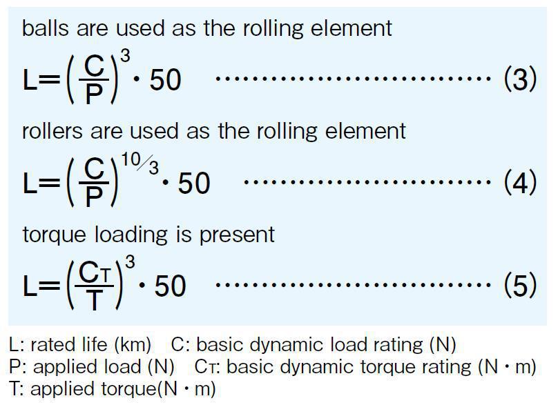
The rated life estimation depends on the type of rolling element. Equations (3) and (4) are used for the ball element and for the roller element, respectively. Equation (5) is used when torque loading is present.
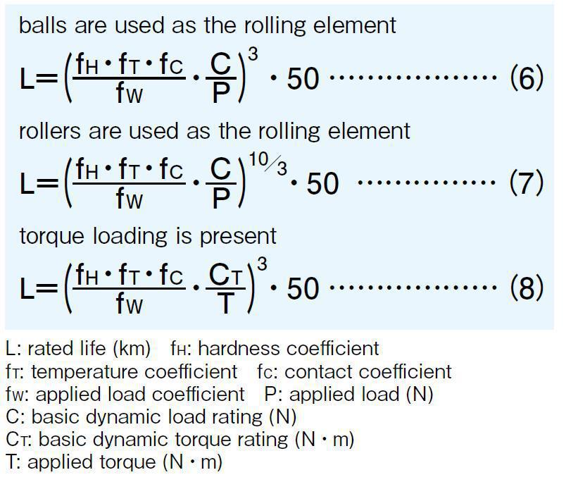
In the actual application, numerous variable factors are present such as in guide rail/shaft accuracy, in mounting conditions, in operating conditions, vibration, and shock, etc. Therefore, calculating the actual applied load accurately is extremely difficult. In general, the calculation is simplified by using coefficients representing these factors: hardness coefficient (fH), temperature coefficient (fT), contact coefficient (fC), and applied load coefficient (fW). Taking these coefficients into account, Equations (3) to (5) become Equations (6) to (8).
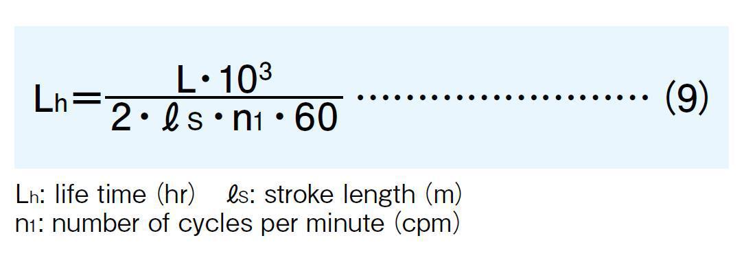
When the travel distance per unit time is constant, the rated life can be expressed in terms of time (hour). Equation (9) shows the relationship between stroke length, number of cycles per minute, and the lifetime.
Hardness Coefficient(fH)
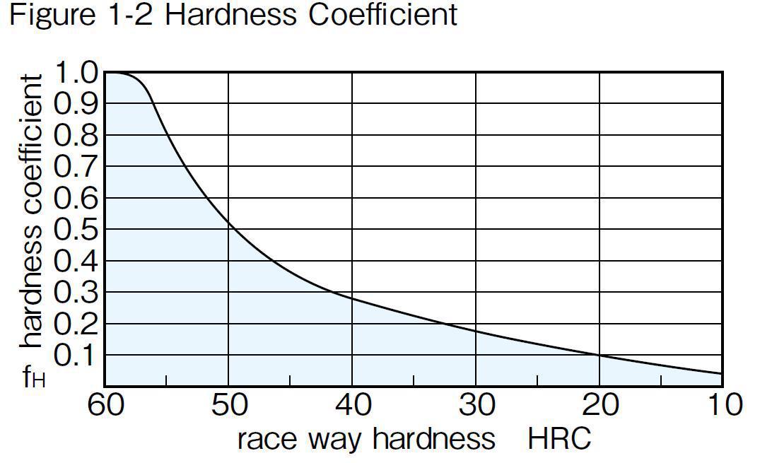
In the linear system, the guide rail or shaft works as a raceway of the rolling elements. Therefore, the hardness of the rail or shaft is an important factor for determining the rated load. The rated load decreases as the hardness decrease below 58HRC. NB products hold appropriate hardness by employing advanced heat treatment technology. In case of using the rail or shaft of insufficient hardness, please take the hardness coefficient (the right figure) into the life calculation equation.
Temperature Coefficient(fT)
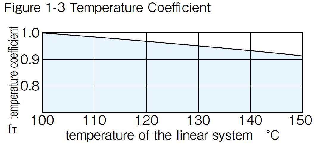
In order to give low wear characteristics, NB products are hardened by heat treatment. If the temperature of the linear system exceeds 100℃, the hardness is decreased by tempering effect and as the rated load decreases. the right figure shows the temperature coefficient as hardness changes with temperature.
Contact Coefficient(fC)
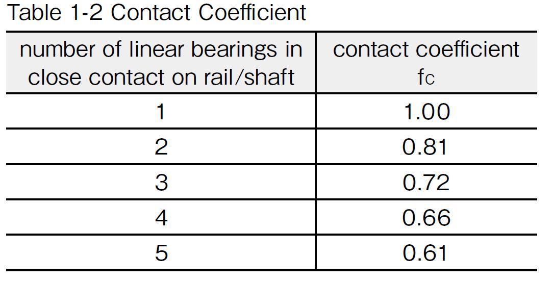
When more than one bearing is used in close contact, the contact coefficient should be taken into consideration due to the variation of products and the accuracy of the mounting surface. The right table shows the contact coefficient for life calculation.
Applied Load Coefficient(fW)
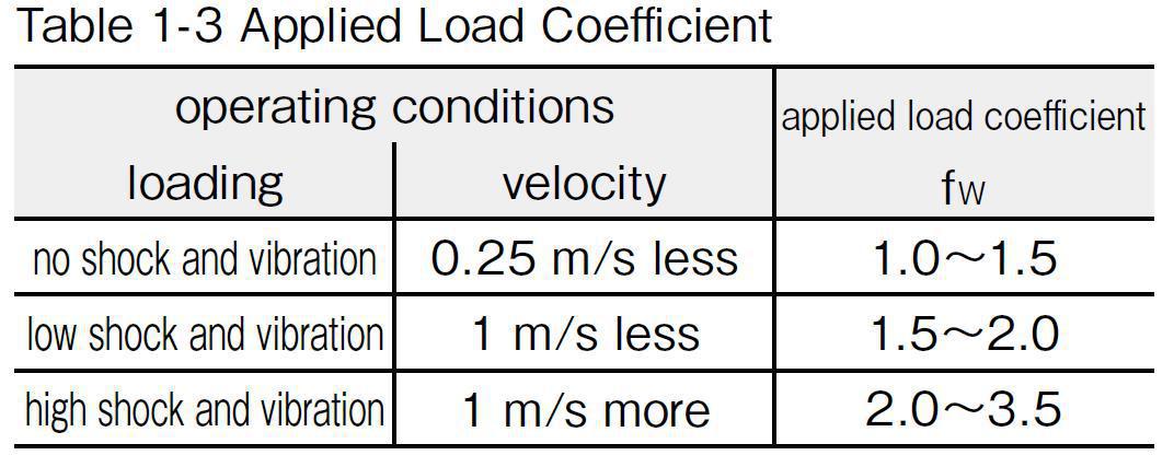
When calculating the applied load, the weight of the mass, inertial force, moment resulting from the motion, and the variation with time should be accurately estimated. However, it is very difficult to accurately estimate the applied load due to the existence of numerous variables, including the start/stop conditions of the reciprocating motion and of the shock/vibration. Estimation is simplified by using the values given in the table.
Calculation of Applied Load(1)
The tables below show the formulas of applied load calculation for typical applications.
W: applied load (N) P1 – P4: load applied to linear system (N) X,Y: linear system span (mm)
x, y, ![]() : distance to applied load or to working center of gravity (mm) g: gravitational acceleration (9.8 x 103mm/s2)
: distance to applied load or to working center of gravity (mm) g: gravitational acceleration (9.8 x 103mm/s2)
V: velocity (mm/s) t1: acceleration time (sec) t3: deceleration time (sec)
Under static conditions or constant velocity motion
|
2 horizontal axes
|
applied load calculation formula
|
 |
 |
|
2 horizontal axes,over-hang
|
applied load calculation formula
|
 |
|
|
2 horizontal axes,moving axes
|
applied load calculation formula
|
 |
|
|
2 horizontal, side axes
|
applied load calculation formula
|
 |
 |
|
2 vertical axes
|
applied load calculation formula
|
 |
 |
Under constant acceleration conditions
|
2 horizontal axes
|
applied load calculation formula
|
 |
 |
Equivalent Coefficient
The linear systems are generally used with two axes, each axis with a couple of bearings installed. However, due to a space limitation, there must be an application in which one axis with one or two bearings in close contact installed. In such a case, multiply the applied moment by the equivalent moment coefficient shown in the appended table for applied load calculation. The following is a formula for calculating the equivalent moment load when a moment is applied to the linear system.
P: equivalent moment load per bearing(N)
E: equivalent moment coefficient
M: applied moment(N・mm)
Calculation of Applied Load(2)
The tables below shows the formulas for determining the applied load when moment is applied to the linear system.
W: applied load (N) P: load applied to the linear system (N) ![]() : distance to applied load or to working center of gravity (mm)
: distance to applied load or to working center of gravity (mm)
Single axis application
|
1 horizontal axis,1 bearing
|
applied load calculation formula
|
 |
|
|
1 sideway axis,1 bearing
|
applied load calculation formula
|
 |
 |
|
1 vertical axis,1 bearing
|
applied load calculation formula
|
 |
 |
2 axes application
|
2 horizontal axes,1 bearing each
|
applied load calculation formula
|
 |
 |
|
2 sideway axes,1 bearing each
|
applied load calculation formula
|
 |
 |
|
2 vertical axes,1 bearing each
|
applied load calculation formula
|
 |
 |
Average Applied Load
The load applied to a linear system generally varies with the travel distance depending on how the system is operated. This includes the start/stop processes of the reciprocating motion and work on the system. The average applied load is used to compute the life corresponding to the actual application conditions.
When the load varies in a step manner with the travel distance
![]() 1 is the travel distance under load
1 is the travel distance under load
![]() 2 is the travel distance under load
2 is the travel distance under load
![]() n is the travel distance under load Pn
n is the travel distance under load Pn
The average applied load Pm is obtained by the following equation.
Pm: average applied load (N)
![]() : total travel distance (m)
: total travel distance (m)
When the applied load varies linearly with the travel distance
The average applied load Pm is a p proximated by the following equation.
Pmin: minimum applied load (N)
Pmax: maximum applied load (N)
When the applied load draws a sine-curve as shown by the right figure (a) and (b)
The average applied load Pm is approximated by the following equations.